Examples#
Temporal Tissue Dynamics from a Spatial Snapshot (Somer, Mannor, Alon, 2025.)#
The following notebooks reproduce the main results from the paper. Notebook names and functions match figure indices in the paper.
Note
Some notebooks download data and perform computationally intensive operations that may take several minutes to complete.
Plot Gallery#
Below you’ll find code samples that produce specific plots.
Each notebook starts by loading a cached Analysis object.
Hint
Run the following code to fit and cache an Analysis that reproduces the fibroblast-macrophage dynamics
from Figure 3 of the paper by Somer et.al 2024
Note: You can skip this if you cached an analysis in the One-shot dynamics in 7 minutes tutorial.
from tdm.raw.breast_mibi import read_single_cell_df
from tdm.cell_types import FIBROBLAST, MACROPHAGE, TUMOR, ENDOTHELIAL
from tdm.analysis import Analysis
from tdm.plot.two_cells.phase_portrait import plot_phase_portrait

# 1. read the single cell dataframe:
single_cell_df = read_single_cell_df()

# 2. fit the analysis:
ana = Analysis(
   single_cell_df=single_cell_df,
   cell_types_to_model=[FIBROBLAST, MACROPHAGE],
   allowed_neighbor_types=[FIBROBLAST, MACROPHAGE, TUMOR, ENDOTHELIAL],
   polynomial_dataset_kwargs={"degree":2},
   neighborhood_mode='extrapolate',
)

# 3. cache the analysis:
ana.dump('fm.pkl')
To load a cached analysis you then run:
ana = Analysis.load('fm.pkl')
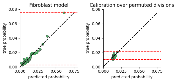
Evaluating a Model#
Calibration
The calibration plots are a good way to test whether neighborhood composition explains the variance in cell division rate.
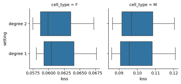
Cross Validation
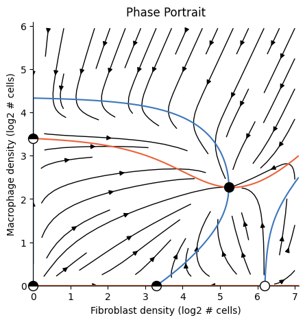
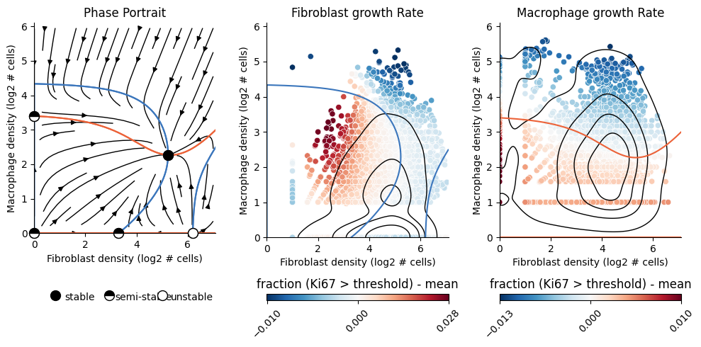
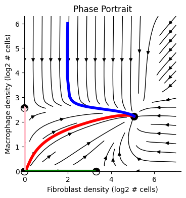
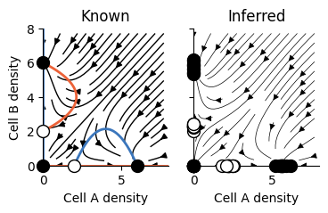
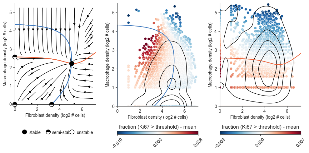
2D Dynamics#
2D Phase-portrait